Seyedali Mirjalili

Salp Swarm Algorithm

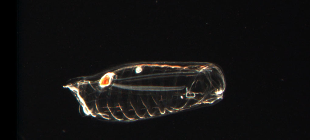
Salps belong to the family of Salpidae and have transparent barrel-shaped body. Their tissues are highly similar to jelly fishes. They also move very similar to jelly fish, in which the water is pumped through body as propulsion to move forward [1]. The shape of a salp is shown below:

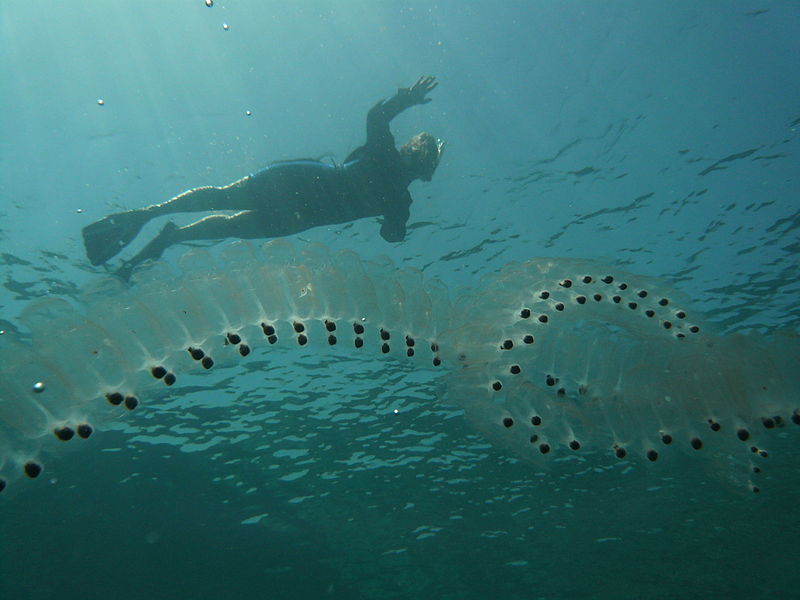
The biological researches about this creature is in its early milestones mainly because their living environments are extremely difficult to access, and it is really difficult to keep them in laboratory environments. One of the most interesting behaviour of salps, which is of interest in the paper, is their swarming behaviour. In deep oceans, salps often form a swarm called salp chain. This chain is illustrated in Fig. 1(b). The main reason of this behaviour is not very clear yet, but some researchers believe that this is done for achieving better locomotion using rapid coordinated changes and foraging [1].

There is little in the literature to mathematically model the swarming behaviours [2] and population of salps [3]. In addition, there is no mathematical model of salp swarms for solving optimization problems while swarms of bees, ants, and fishes have been widely modelled and used for solving optimization problems. This subsection proposes the first model of salp chains in the literature for the purpose of solving optimization problems.
To mathematically model the salp chains, the population is first divided to two groups: leader and followers. The leader is the salp at the front of the chain, whereas the rest of salps are considered as followers. As the name of these salps implies, the leader guides swarm and the followers follow each other (and leader directly of indirectly).
Similarly to other swarm-based techniques, the position of salps is defined in an n-dimensional search space where n is the number of variables of a given problem. Therefore, the position of all salps are stored in a two-dimensional matrix called x. It is also assumed that there is a food source called F in the search space as the swarm’s target.

To update the positon of the leader the following equation is proposed:

where x_j^1 shows the position of the first salp (leader) in the j-th dimension, F_j is the position of the food source in the j-th dimension, ub_j indicates the upper bound of j-th dimension, lb_j indicates the lower bound of j-th dimension, c_1, c_2, and c_3 are random numbers.

The above equation shows that the leader only updates its position with respect to the food source. The coefficient c_1 is the most important parameter in SSA because it balances exploration and exploitation defined as follows:

where l is the current iteration and L is the maximum number of iterations.

The parameter c_2 and c_3 are random numbers uniformly generated in the interval of [0,1]. In fact, they dictate if the next position in j-th dimension should be towards positive infinity or negative infinity as well as the step size.
To update the position of the followers, the following equations is utilized (Newton’s law of motion):

were i≥2, x_j^i shows the position of i-th follower salp in j-th dimension, t is time, v_0 is the initial speed, and a is calculated as follows:

Because the time in optimization is iteration, the discrepancy between iterations is equal to 1, and considering v_0=0, this equation can be expressed as follows:

where i≥2 and x_j^i shows the position of i-th follower salp in j-th dimension.

With Eqs. (3.1) and (3.4), the salp chains can be simulated.

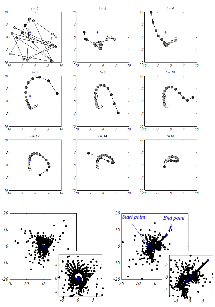
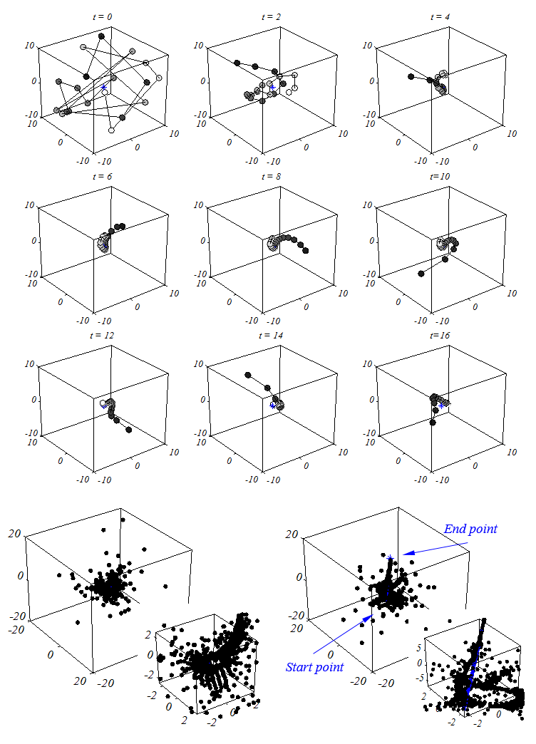
In order to see the effects of the above mathematical model proposed, a simulation is done in this subsection. Twenty salps are randomly placed on a search space with stationary or moving sources of food. The position of the salp chains and history of each salp are drawn in the following figures.. Note that the blue point in the figures shows the position of food source and the darkest filled circle is the leading salp. The follower salps are coloured with grey based on their position in the salp chain with respect to the leader. Inspecting the behaviour of salp chain over nine consecutive iterations. it may be observed that the swarm can be formed and moved using the equation proposed effectively right after the first iteration. Also, it can be seen that the leading salp changes its position around the food source and follower salps gradually follow it over the course of iterations. The same model has been utilized for both simulations and the merits of the model proposed in both 2D and 3D spaces are evident in the figures. It can be stated that the model is able to show the same behaviour in an n-dimensional space.

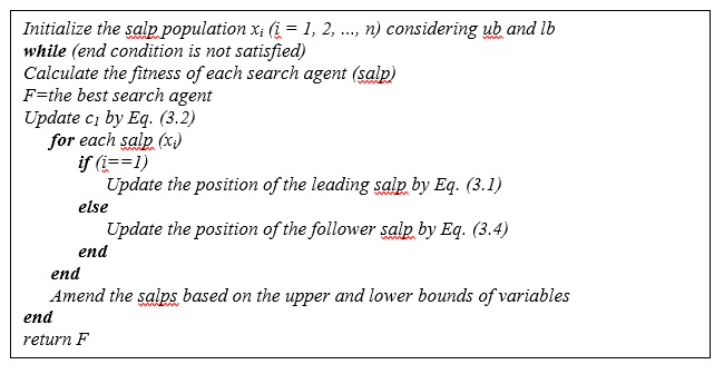
The pseudo code of the SSA algorithm is illustrated below. This figure shows that the SSA algorithm starts approximating the global optimum by initiating multiple salps with random positions. It then calculates the fitness of each salp, finds the salp with the best fitness, and assigns the position of the best salp to the variable F as the source food to be chased by the salp chain. Meantime the coefficient c1 is updated.. For each dimension, the position of leading salp is updated and the position of follower salps are updated. If any of the salp goes outside the search space, it will be brought back on the boundaries. All the above steps except initialization are iteratively executed until the satisfaction of an end criterion.

.It should be noted that the food source will be updated during optimization because the salp chain is very likely to find a better solution by exploring and exploiting the space around it. The above simulations show that the salp chain modelled is able to chase a moving food source. Therefore, the salp chain has the potential to move towards the global optimum that changes over the course of iterations. To see how the proposed salp chain model and SSA algorithm are effective in solving optimization problems, some remarks are listed as follows:

•    SSA algorithm saves the best solution obtained so far and assigns it to the food source variable, so it never get lost even if the whole population deteriorates.
•    SSA algorithm updates the position of the leading salp with respect to the food source only, which is the best solution obtained so far, so the leader always explores and exploits the space around it.
•    SSA algorithm updates the position of follower salps with respect to each other, so they move gradually towards the leading salp.
•    Gradual movements of follower slaps prevent the SSA algorithm from easily stagnating in local optima.
•    Parameter c1 is decreased adaptively over the course of iterations, so the SSA algorithm first explores the search space and then exploits it.
•    SSA algorithm has only one main controlling parameter (c1).
•    SSA algorithm is simple and easy to implement.

These remarks make the SSA algorithm theoretically and potentially able to solve single-objective optimization problems with unknown search spaces. The adaptive mechanism of SSA allows this algorithm to avoid local solutions and eventually finds an accurate estimation of the best solution obtained during optimization. Therefore, it can be applied to both unimodal and multi-modal problems. The above-mentioned advantages potentially allow SSA to outperform recent algorithms (GWO, ABC, etc). However, this cannot be guaranteed for all optimization problems according to the NFL theorem

Note that the computational complexity of the SSA algorithm is of O(t(d*n + Cof*n)) where t shows the number of iterations, d is the number of variables (dimension), n is the number of solutions, and Cof indicates the cost of objective function.

The source code of SSA is publicly avaiable here to download:

You can download the paper here.

If you have no access to Sciencedirect, drop me an e-mail here and I will send you the paper. Please also do not hesitate to contact me for any questions and criticisms. I am always happy to hear your thoughts.

If you have any questions or something to share, please feel free to post it at the end of this page in the comment section.

References

[1]    P. A. Anderson and Q. Bone, "Communication between individuals in salp chains II. Physiology," Proceedings of the Royal Society of London B: Biological Sciences, vol. 210, pp. 559-574, 1980.
[2]    V. Andersen and P. Nival, "A model of the population dynamics of salps in coastal waters of the Ligurian Sea," Journal of plankton research, vol. 8, pp. 1091-1110, 1986.
[3]    N. Henschke, J. A. Smith, J. D. Everett, and I. M. Suthers, "Population drivers of a Thalia democratica swarm: insights from population modelling," Journal of Plankton Research, p. fbv024, 2015.